Raman Lidars#
The first MPI-M Raman lidar deployed at BCO in April 2010 was the EARLI system. EARLI ran for the first six years of site operation, positioned a few meters from the seashore.
In 2016 EARLI was replaced with LICHT (LIdar for Cloud, Humidity and Temperature profiling). LICHT has similar measurement characteristics to EARLI and was not designed for outdoor use. LICHT was on board the German research ship METEOR during the EUREC4A field campaign in January and February of 2020.
The CORAL system (Cloud Observation with Radar And Lidar) is the third-generation MPI-M Raman lidar at BCO, dedicated primarily to high resolution water vapor vertical profiling. CORAL began operating at BCO in May 2019.
Examples#
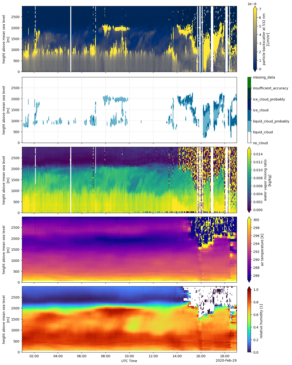
Cold pool passage over the BCO#
This an example plotting several quantities available from the Raman lidar CORAL for a date when several cold pools from a flower mesoscale system were detected from the BCO. The detection was performed by [Vogel et al., 2021] using surface temperature measurements. This example was taken from Figure 2 in the paper.
import intake
import matplotlib.pylab as plt
import matplotlib.ticker as ticker

cat = intake.open_catalog("https://tcodata.mpimet.mpg.de/catalog.yaml")

# Load fast and slow products
coral_lidar_b = cat.BCO.lidar_CORAL_LR_b_c1_v1.to_dask()
coral_lidar_t = cat.BCO.lidar_CORAL_LR_t_c1_v1.to_dask()

# Time period from first plot in the paper
start_time = "2020-02-29T01:00"
end_time = "2020-02-29T19:00"

# Select region of interest
region = {"time": slice(start_time, end_time), "alt": slice(0,3000)}
coral_lidar_b = coral_lidar_b.sel(**region)
coral_lidar_t = coral_lidar_t.sel(**region)

# Plot lidar data
fig, axes = plt.subplots(5, sharex=True, sharey=True, figsize=(12, 15), constrained_layout=True)

# Backscatter
coral_lidar_b.bp532.plot(x="time", vmin=0, vmax=7e-6, ax=axes[0], cmap="cividis")

# Cloud mask (flag variables), setting missing values to nan
cloudmask = coral_lidar_b.cloud_mask
cloudmask = cloudmask.where(cloudmask<5)
im = cloudmask.plot.contourf(x="time", vmin=-0.5, vmax=4.5, ax=axes[1],
                        cmap="ocean_r", add_colorbar=False)
ticks = cloudmask.flag_values
labels = cloudmask.flag_meanings.split(" ")
cbar = fig.colorbar(im, ax=axes[1])
#cbar.set_ticks(ticks)
cbar.ax.set_yticklabels(labels)
axes[1].grid(alpha=0.3)

# Mixing ratio
coral_lidar_b.mr.plot(x="time", vmin=0, vmax=15e-3, ax=axes[2], cmap="viridis")

# Temperature
coral_lidar_t.ta.plot(x="time", vmin=285, vmax=300, ax=axes[3], cmap="plasma")

# Relative Humidity
coral_lidar_t.rh.plot(x="time", vmin=0, vmax=1, ax=axes[4], cmap="turbo")

# Beautify axis
for ax in axes[:-1]:
    ax.set_xlabel("")

axes[-1].set_xlabel("UTC Time");
/builds/tco/bco/docs/.venv/lib/python3.12/site-packages/intake_xarray/base.py:21: FutureWarning: The return type of `Dataset.dims` will be changed to return a set of dimension names in future, in order to be more consistent with `DataArray.dims`. To access a mapping from dimension names to lengths, please use `Dataset.sizes`.
  'dims': dict(self._ds.dims),