Cloud Radars

Cloud radars use electromagnetic radiation approximately in the range of 30 to 200 GHz in bands which are sensitive to cloud droplets and ice crystals. As the wavelength is typically larger than the size of the observed particles, the signal is mainly governed by Rayleigh scattering, and thus, the signal is more sensitive to the size of the observed particles than their amount. Although clouds attenuate the radiation, cloud radars can typically see through clouds and thus, can also provide information behind the first layer.

A radar from the Karlsruhe Institute of Technology (KIT) inaugurated the long lineage of BCO Ka-band radars in 2010, after which the KATRIN radar arrived in December of the same year, replacing the KIT radar soon after. In 2015, the MBR2 replaced the KATRIN radar, and it enjoyed a lengthy tenure before it was decomissioned in 2024. As it was phased out, the MBRS radar began operations, and this radar is still in operation.

At the end of 2018, a W Band radar (called RUMBA) was installed and has since been in operation intermittently with a large hiatus from September 2024 to January 2026.

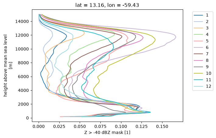
A level 2 product on the vertical axis of the MBRS and of the fourth configuration of MBR2 can be accessed as shown below. The dataset contains rabbit-ear filtered reflectivities and selected level 1 variables, with an added cloud_fraction defined as reflectivities greater than -40 dBZ. We drop low transmission power, and we set reflectivities with signals below the instrument’s sensitivity threshold to -inf, whereas we set reflectivities above the instrument’s sensitivity threshold to +inf. The dataset is available at a range of time resolutions.

import intake
cat = intake.open_catalog("https://tcodata.mpimet.mpg.de/catalog.yaml")
ds = cat.BCO.cloudradar(time="PT1H").to_dask()
ds

/builds/tco/bco/docs/.venv/lib/python3.14/site-packages/intake_xarray/base.py:21: FutureWarning: The return type of `Dataset.dims` will be changed to return a set of dimension names in future, in order to be more consistent with `DataArray.dims`. To access a mapping from dimension names to lengths, please use `Dataset.sizes`.
  'dims': dict(self._ds.dims),

<xarray.Dataset> Size: 7GB
Dimensions:         (time: 138630, alt: 605, bnd: 2)
Coordinates:
  * time            (time) datetime64[ns] 1MB 2010-12-22T19:30:00 ... 2026-10...
  * alt             (alt) float64 5kB 174.4 205.6 236.8 ... 1.898e+04 1.901e+04
    lat             float64 8B ...
    lon             float64 8B ...
Dimensions without coordinates: bnd
Data variables: (12/13)
    DPS             (time, alt) float64 671MB dask.array<chunksize=(131072, 32), meta=np.ndarray>
    DPSwav          (time, alt) float64 671MB dask.array<chunksize=(131072, 32), meta=np.ndarray>
    LDR             (time, alt) float64 671MB dask.array<chunksize=(131072, 32), meta=np.ndarray>
    MeltHei         (time) float32 555kB dask.array<chunksize=(138630,), meta=np.ndarray>
    NPK             (time, alt) float64 671MB dask.array<chunksize=(131072, 32), meta=np.ndarray>
    RHO             (time, alt) float64 671MB dask.array<chunksize=(131072, 32), meta=np.ndarray>
    ...              ...
    SNR             (time, alt) float64 671MB dask.array<chunksize=(131072, 32), meta=np.ndarray>
    VEL             (time, alt) float64 671MB dask.array<chunksize=(131072, 32), meta=np.ndarray>
    Z               (time, alt) float64 671MB dask.array<chunksize=(131072, 32), meta=np.ndarray>
    cloud_fraction  (time, alt) float64 671MB dask.array<chunksize=(131072, 32), meta=np.ndarray>
    raw_count       (time) float64 1MB dask.array<chunksize=(138630,), meta=np.ndarray>
    time_bounds     (time, bnd) datetime64[ns] 2MB dask.array<chunksize=(138630, 2), meta=np.ndarray>
Attributes:
    Conventions:           CF-1.12
    _cutoff_date:          2026-10-16T00:00:04.000001000
    _logical_cutoff_date:  2014-11-01T00:00:00Z
    bcoproc_version:       0.0.0.post2354.dev0+f9b7f57e
    featureType:           timeSeriesProfile
    institution:           Max Planck Institute for Meteorology, Hamburg
    license:               CC-BY-4.0
    location:              The Barbados Cloud Observatory (BCO), Deebles Poin...
    platform:              BCO
    source:                https://swift.dkrz.de/v1/dkrz_948e7d4bbfbb445fbff5...
    title:                 Ka-band cloud radar data (level 2, rabbit-ear filt...
    tool_versions:         {"Python": "3.14.3 (main, Mar  3 2026, 14:59:53) [...

xarray.Dataset

• Dimensions:
  • time: 138630
  • alt: 605
  • bnd: 2
• Coordinates: (4)
  • time
    (time)
    datetime64[ns]
    2010-12-22T19:30:00 ... 2026-10-...

    axis :

    T

    standard_name :

    time

    units_metadata :

    leap_seconds: utc

    array(['2010-12-22T19:30:00.000000000', '2010-12-22T20:30:00.000000000',
           '2010-12-22T21:30:00.000000000', ..., '2026-10-15T22:30:00.000000000',
           '2026-10-15T23:30:00.000000000', '2026-10-16T00:30:00.000000000'],
          shape=(138630,), dtype='datetime64[ns]')

  • alt
    (alt)
    float64
    174.4 205.6 ... 1.898e+04 1.901e+04

    axis :

    Z

    long_name :

    height above mean sea level

    positive :

    up

    standard_name :

    altitude

    units :

    m

    array([  174.4 ,   205.58,   236.75, ..., 18944.28, 18975.45, 19006.63],
          shape=(605,))

  • lat
    ()
    float64
    ...

    [1 values with dtype=float64]

  • lon
    ()
    float64
    ...

    [1 values with dtype=float64]

• Data variables: (13)
  • DPS
    (time, alt)
    float64
    dask.array<chunksize=(131072, 32), meta=np.ndarray>

    cell_methods :

    time: circmean

    db :

    0

    long_name :

    Differential Phase

    units :

    deg

    yrange :

    [-180.0, 180.0]

    Array Chunk Bytes 639.89 MiB 32.00 MiB Shape (138630, 605) (131072, 32) Dask graph 38 chunks in 2 graph layers Data type float64 numpy.ndarray

  • DPSwav
    (time, alt)
    float64
    dask.array<chunksize=(131072, 32), meta=np.ndarray>

    cell_methods :

    time: circmean

    db :

    0

    long_name :

    Differential Phase peak weighted

    units :

    deg

    yrange :

    [-180.0, 180.0]

    Array Chunk Bytes 639.89 MiB 32.00 MiB Shape (138630, 605) (131072, 32) Dask graph 38 chunks in 2 graph layers Data type float64 numpy.ndarray

  • LDR
    (time, alt)
    float64
    dask.array<chunksize=(131072, 32), meta=np.ndarray>

    applied_thresholds :

    dBZ < -35 between 1000m and 8000m, with instrument-dependent Doppler vel. thresholds

    cell_methods :

    time: logmean

    db :

    1

    details :

    artifacts (rabbit-ears), caused by side lobes, are removed

    long_name :

    linear de-polarization ratio LDR of all hydrometeors

    units :

    dB

    valid_range :

    [-35.0, 5.0]

    Array Chunk Bytes 639.89 MiB 32.00 MiB Shape (138630, 605) (131072, 32) Dask graph 38 chunks in 2 graph layers Data type float64 numpy.ndarray

  • MeltHei
    (time)
    float32
    dask.array<chunksize=(138630,), meta=np.ndarray>

    cell_methods :

    time: mean

    db :

    0

    long_name :

    melting layer height

    units :

    m

    valid_range :

    [0, 14000]

    Array Chunk Bytes 541.52 kiB 541.52 kiB Shape (138630,) (138630,) Dask graph 1 chunks in 2 graph layers Data type float32 numpy.ndarray

  • NPK
    (time, alt)
    float64
    dask.array<chunksize=(131072, 32), meta=np.ndarray>

    cell_methods :

    time: logmean

    db :

    0

    long_name :

    Number of Peaks

    units :

    yrange :

    [-1, 10]

    Array Chunk Bytes 639.89 MiB 32.00 MiB Shape (138630, 605) (131072, 32) Dask graph 38 chunks in 2 graph layers Data type float64 numpy.ndarray

  • RHO
    (time, alt)
    float64
    dask.array<chunksize=(131072, 32), meta=np.ndarray>

    cell_methods :

    time: mean

    db :

    0

    long_name :

    Co-Cross Channel Correlation

    units :

    yrange :

    [0.0, 1.0]

    Array Chunk Bytes 639.89 MiB 32.00 MiB Shape (138630, 605) (131072, 32) Dask graph 38 chunks in 2 graph layers Data type float64 numpy.ndarray

  • RHOwav
    (time, alt)
    float64
    dask.array<chunksize=(131072, 32), meta=np.ndarray>

    cell_methods :

    time: mean

    db :

    0

    long_name :

    Cross Channel Correlation Peak weighted

    units :

    yrange :

    [0.0, 1.0]

    Array Chunk Bytes 639.89 MiB 32.00 MiB Shape (138630, 605) (131072, 32) Dask graph 38 chunks in 2 graph layers Data type float64 numpy.ndarray

  • SNR
    (time, alt)
    float64
    dask.array<chunksize=(131072, 32), meta=np.ndarray>

    applied_thresholds :

    dBZ < -35 between 1000m and 8000m, with instrument-dependent Doppler vel. thresholds

    cell_methods :

    time: logmean

    db :

    1

    details :

    artifacts (rabbit-ears), caused by side lobes, are removed

    long_name :

    reflectivity SNR

    units :

    dB

    valid_range :

    [-28.597850799560547, 80.0]

    Array Chunk Bytes 639.89 MiB 32.00 MiB Shape (138630, 605) (131072, 32) Dask graph 38 chunks in 2 graph layers Data type float64 numpy.ndarray

  • VEL
    (time, alt)
    float64
    dask.array<chunksize=(131072, 32), meta=np.ndarray>

    cell_methods :

    time: mean

    db :

    0

    long_name :

    doppler velocity VEL of all hydrometeors

    units :

    m s-1

    valid_range :

    [-10.5563383102417, 10.5563383102417]

    Array Chunk Bytes 639.89 MiB 32.00 MiB Shape (138630, 605) (131072, 32) Dask graph 38 chunks in 2 graph layers Data type float64 numpy.ndarray

  • Z
    (time, alt)
    float64
    dask.array<chunksize=(131072, 32), meta=np.ndarray>

    applied_thresholds :

    dBZ < -35 between 1000m and 8000m, with instrument-dependent Doppler vel. thresholds

    cell_methods :

    time: logmean

    db :

    1

    details :

    artifacts (rabbit-ears), caused by side lobes, are removed

    long_name :

    equivalent radar reflectivity of all hydrometeors

    units :

    dBZ

    valid_range :

    [-60.0, 30.0]

    Array Chunk Bytes 639.89 MiB 32.00 MiB Shape (138630, 605) (131072, 32) Dask graph 38 chunks in 2 graph layers Data type float64 numpy.ndarray

  • cloud_fraction
    (time, alt)
    float64
    dask.array<chunksize=(131072, 32), meta=np.ndarray>

    applied_thresholds :

    dBZ < -35 between 1000m and 8000m, with instrument-dependent Doppler vel. thresholds

    cell_methods :

    time: mean

    db :

    1

    details :

    artifacts (rabbit-ears), caused by side lobes, are removed

    long_name :

    Z > -40 dBZ mask

    units :

    1

    valid_range :

    [0, 1]

    Array Chunk Bytes 639.89 MiB 32.00 MiB Shape (138630, 605) (131072, 32) Dask graph 38 chunks in 2 graph layers Data type float64 numpy.ndarray

  • raw_count
    (time)
    float64
    dask.array<chunksize=(138630,), meta=np.ndarray>

    cell_methods :

    time: sum

    Array Chunk Bytes 1.06 MiB 1.06 MiB Shape (138630,) (138630,) Dask graph 1 chunks in 2 graph layers Data type float64 numpy.ndarray

  • time_bounds
    (time, bnd)
    datetime64[ns]
    dask.array<chunksize=(138630, 2), meta=np.ndarray>

    Array Chunk Bytes 2.12 MiB 2.12 MiB Shape (138630, 2) (138630, 2) Dask graph 1 chunks in 2 graph layers Data type datetime64[ns] numpy.ndarray

• Attributes: (12)

  Conventions :

  CF-1.12

  _cutoff_date :

  2026-10-16T00:00:04.000001000

  _logical_cutoff_date :

  2014-11-01T00:00:00Z

  bcoproc_version :

  0.0.0.post2354.dev0+f9b7f57e

  featureType :

  timeSeriesProfile

  institution :

  Max Planck Institute for Meteorology, Hamburg

  license :

  CC-BY-4.0

  location :

  The Barbados Cloud Observatory (BCO), Deebles Point, Barbados, West Indies

  platform :

  BCO

  source :

  https://swift.dkrz.de/v1/dkrz_948e7d4bbfbb445fbff5315fc433e36a/airflow_production/BCO.cloudradar_x8c970f_0_PT10M.zarr

  title :

  Ka-band cloud radar data (level 2, rabbit-ear filtered) from the BCO

  tool_versions :

  {"Python": "3.14.3 (main, Mar 3 2026, 14:59:53) [Clang 21.1.4 ]", "idna": "3.20", "frozenlist": "1.8.0", "charset_normalizer": "3.5.2", "tzdata": "2026.5", "bcoproc": "0.0.0.post2354.dev0+f9b7f57e", "datarecords": "0.0.0.post2354.dev0+f9b7f57e", "asciitree": "0.3.3", "locket": "1.0.0", "partd": "1.4.2", "cftime": "1.6.6", "certifi": "2026.7.22", "numcodecs": "0.15.1", "multidict": "6.9.1", "numpy": "2.5.3", "cloudpickle": "3.1.2", "toolz": "1.2.0", "urllib3": "2.8.0", "packaging": "26.3", "iniconfig": "2.3.1", "scipy": "1.18.1", "fsspec": "2026.9.0", "ruff": "0.13.0", "xarray": "2026.7.0", "six": "1.17.0", "requests": "2.34.2", "pendulum": "3.2.0", "appdirs": "1.4.4", "deprecated": "3.0.0", "attrs": "26.1.0", "intake": "0.7.0", "netcdf4": "1.7.4", "pandas": "3.0.6", "wrapt": "2.5.0", "bcologs": "0.0.0.post2354.dev0+f9b7f57e", "zarr": "2.18.7", "pyyaml": "6.0.3", "msgpack": "1.2.3", "aiosignal": "1.4.0", "pluggy": "1.6.0", "pytest": "9.1.1", "entrypoints": "0.4", "aiohappyeyeballs": "2.7.1", "netCDF4": "1.7.4", "numpy_groupies": "0.12.3", "aiohttp": "3.14.4", "setuptools": "84.0.0", "yarl": "1.25.1", "click": "8.5.0", "propcache": "0.5.4", "pyzstd": "0.19.1", "jinja2": "3.1.6", "pygments": "2.21.0", "flox": "0.11.2", "dask": "2026.8.0", "MarkupSafe": "3.0.4", "python-dateutil": "2.9.0.post0"}

monthly cloud fraction profiles

Show code cell content

Hide code cell content

import numpy as np
import matplotlib.pyplot as plt
months = np.unique(ds.time.dt.month)
colors = [tuple(color) for color in plt.get_cmap("tab20")(np.linspace(0, 1, len(np.unique(ds.time.dt.month))))]

for m in months:
    ds.sel(time=ds.time.dt.month.isin([m]), alt=slice(None, 15000)).cloud_fraction.mean(dim="time").plot(y="alt", label=m, color=colors[m-1])
plt.legend(bbox_to_anchor=(1.05, 1), loc='upper left')

<matplotlib.legend.Legend at 0x7fec5801e270>